EKF SLAM from Scratch

Project Goal

The objective of this project is to create an EKF SLAM algorithm from scratch to understand the mathematical theory behind SLAM algorithms, the structure of coding a Kalman filter in C++, and nuances between simulation in Rviz and deploying on the turtlebot3 burger. This is a feature based algorithm that relies on the odometry estimates and landmark measurements to navigate and localize. The linearization of the probabilities using Taylor series approximation is what makes this project approachable in a 10 week scope.

Disclaimer

This project is currently in progress and will be posted in completion later this month.

Approach

Setup

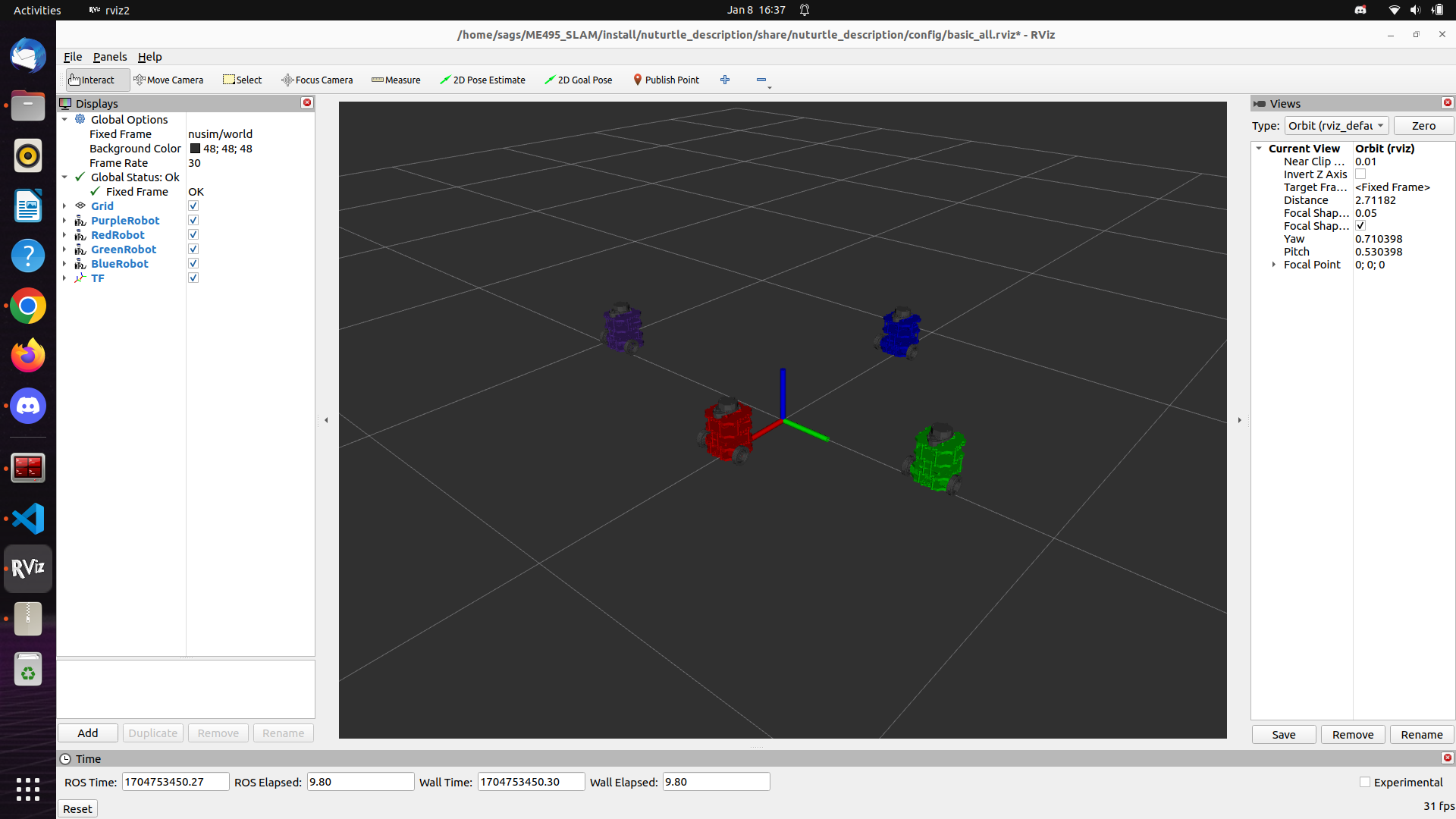
The first steps of this project involved showing the Turtlebot3 burger in simulation in 3 different colors. This allows us to represent a different thing with each robot.

• Red: The red robot represents the “ground truth” when simulating the robots. It moves as if all sensors and commands were perfect with no slip.
• Blue: The blue robot represents the raw odometry meaning it moves exactly as the encoder would have the robot believe but has no sensing abiliity.
• Green: The green robot represents the SLAM estimate of the robot within the environment based on the sensed obstacles and odometry estimates on a small scale.
• Purple: The purple robot is just there for some NU fun and does not appear later in this project.
• Pillars: These pillars are obstacles for the simulation to use as landmarks (shown in later images/videos).

Custom Libraries

In order to make simplify this project, I created many custom libraries to model the geometry conversions, 2D transformations, differential drive motion functionality, and EKF functions to simplify the usage in the slam node.

Odometry and Simulation

Once the robots are modeled, it was necessary to simulate a realistic red robot that can mimic the output of a real Turtlebot3 using all of the same sensor outputs. On top of this I created an odometry node to provide the motion of the blue robot. It is important to know that in simulation the odometry robot will not be affected by obstacles whereas the red will because the encoders will continue to spin and make the blue robot percieve motion. The below image shows the path of the blue vs red robot where the blue goes right through the obstacle.

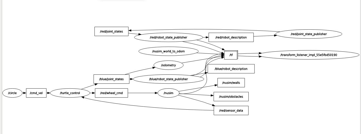
In the graph below, nusim represents the simulation arena for the robots to interact. Turtle_control siginifies the control of the real robot from a commanded velocity into motion of the motors. Circle is a node simply used to publish a command velocity that will have the robot spin in a circle of a given radius at a given speed.

Odometry in real life

Below is a video showing the robot moving in real life vs the blue odometry robot representing the sensed motion from the encoders. It is important to note that the red robot is NOT present in the simulation because the “ground truth” is the real robot. Only the blue robot is there to represent the motion of the odometry.

SLAM and Next Steps

Now that the odometry is modeled, it is time to implement the SLAM algorithm. My EKF library can be summed into two main functions. First is the “predict” function that will use the odometry values and the sensor reading to predict where the robot should be. The next function is the “correct” function that will move the odometry frame to correct the green robot when it deviates from the red/ground truth robot.

Predict

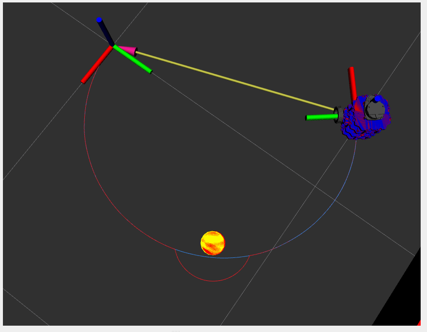
Below is a video showing the initial tests for the “predict” funciton in action. The flashing yellow markers show the simulated noise in the perception of the obstacle from the red robot’s lidar. This is what the green robot uses as landmarks to localize. The white dots simulate the rays from the 2D lidar on the turtlebot. This will be used for the circle fitting on the real robot.

The green robot is seen following the blue robot because it does not yet have the functionality to correct as the red robot deviates from the path, but it does maintain connection with the blue becuase it is predicting correctly based on the odometry. With the correct function in place, the green robot will stay with the red robot even as the red and blue separate showing that it is able to process the landmarks seen in the environment.

Correction

The below video demonstrates the behavior of the turtlebots when the correct function is being used. The green (SLAM) robot following the red (ground truth) robot rather than the blue (odom) robot after encountering an obstacle shows that the SLAM correction works. As seen when the odometry arrows are removed, the green and red paths are coincident rather than the green and blue paths. Furthermore, the axes for the map and odom frames, which begin coincident at the start of the simulation, separate to shows that the map –> odom frame transformation is accounting for the correction created by the EKF SLAM algorithm.

Correction with Simulated Noise

The video below demonstrates the same motion, but now there is added noise to the sensor readings and odometry. The range of the sensor is also limited meaning that the robot can no longer sense all obstacles at once. Here the algorithm is still shown to function and the green odom frame can be seen correcting for the collision.

Source code

Due to this project being in progress, the code cannot be shared at this time.