Frontier Toolbox: Autonomous Exploration

Featured Video

Project Overview

The goal of this project was to create an easy-to-use platform to rapidly prototype frontier exploration algorithms on a robot in various environments with both full and limited field of view sensor data. Through this package, users should be able to easily leverage the provided libraries to generate, cluster, and evaluate frontiers or integrate the provided component functions into their own novel approaches.

There are many frontier algorithms out there, but all of them follow the same pattern:

1. Identify frontier cells that mark the boundary of the known map space.
2. Group or cluster them together to create continuous boundaries for the robot to explore.
3. Plan the robot’s next move by selecting the best place to go.

Using this framework, the provided frontier node follows the general structure in this diagram to make the robot explore using the tools in the frontier toolbox.

Output

This project provides a ROS2 node exhibiting multiple examples of robot exploration by mix-and-matching the various library functions. (skip ahead to featured algorithms). All of my code is written as ament_cmake ROS2 packages that can be downloaded from GitHub and built from source. Through the README, any user should be able to build the packages and then use the lauch files to either run a full simulation or deploy frontier exploration on a real robot. In my case, this was the Clearpath Jackal.

Source code

To view the code or try it out yourself, check out my Github Repository!

Main Software Components

• frontier exploration (frontier_exp_cpp) package
• Robot setup and mapping (robot_mapping) package
• Nav2 action client node (nav_client_cpp) package

Frontier Navigation

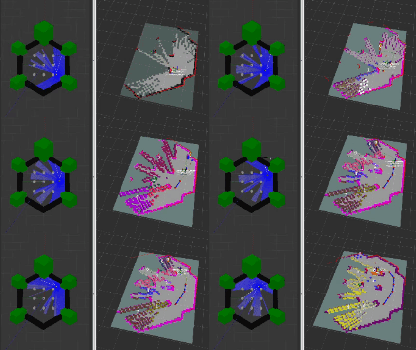
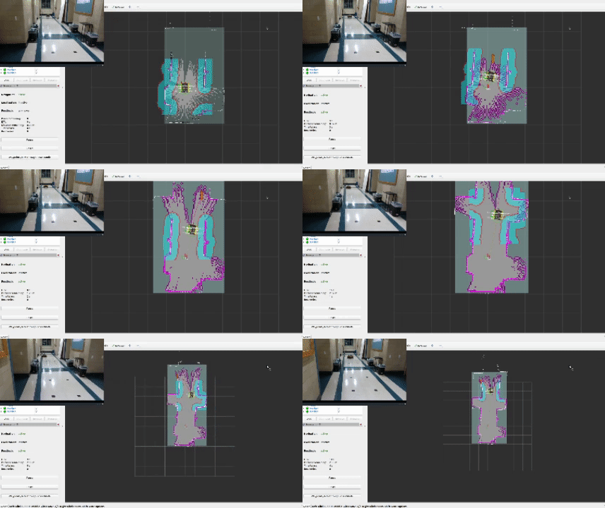
The heart and soul of this project revolves around the frontier navigation package frontier_exp_cpp which exhibits unique frontier exploration algorithms as well as an easy-to-use library of functions to calculate frontiers, clusters, and plan optimal goal positions. When using my frontier_lc lifecycle node, a user can select the algorithm by adjusting parameters in the frontier_params.yaml file. The decision tree is shown below.

Navigation Algorithms

Through the library, many different exploration algorithms were tested by interchanging functions from the general structure diagram. Some of the selected examples are shown below. To see more about the results from this testing, which focused mostly on the scoring of the candidates, feel free to skip ahead to the results section.

Below are featured algorithms tested and included as a part of the frontier_lc lifecycle node. The diagrams below show how mixing and matching can easily construct new algorithms:

• Goal position is the closest single frontier to the robots “viewpoint” which is x[m] in front of the robot. Go to distance approach…
• Goal position is the single frontier with the most information gain/entropy reduction if the robot were to be teleported there. Go to entropy calculation…
• Goal position is the closest cluster centroid after the frontiers have been clustered with DBSCAN. Go to DBSCAN calculation…
• Goal position is the cluster centroid with the most information gain/entropy reduction if the robot were to be teleported there.
• Goal position is the centroid of the cluster with the largest number of frontiers.
• Goal position is the frontier within a sampled set with the most “unknowns flipped” in the state update. See unknown flipping…

Key Computations

Each algorithm relies on key computations allowing the robot to succeed in exploring various environments. Some of the key components that make up the frontier toolbox are the generation of frontiers, the distance based goal selection, the Mutual Information based goal selection, and the DBSCAN clustering algorithm.

Frontier Generation

This approach defines a frontier as a cell that is unknown in the map (-1 in the OccupancyGrid) and is also bordering a cell that is known to be empty (0 in the OccupancyGrid). Since the data is just a 1D array, generating the list of frontiers is O(n). In the image, below, the frontiers are shown on the map in purple. The blue clouds indicate the cost of approaching static objects (occupied cells) shown in pink (100 in the OccupancyGrid).

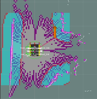
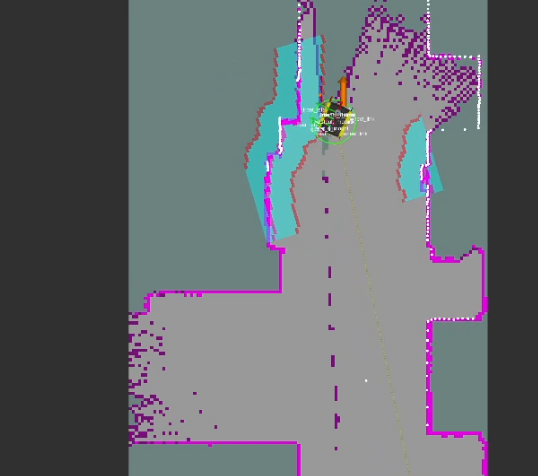
If the map size is large, and the scoring algorithm benefits from a fixed sample size, then a list of frontiers uniformly sampled can be generated and used in place of the full list of frontiers using the provided sample function.

Distance-based Selection

The initial “naive” approach was to have the robot simply select a frontier that is closest to its “viewpoint” which is a point slightly in front of the robot. The purpose of the viewpoint is to encourage the robot to keep moving forward in a greedy depth-first approach. Once the robot hits a dead end, it then selects the next closest frontier. If the robot get’s stuck, this algorithm exploits the “spin” motion in Nav2’s recovery behaviors to hopefully choose a different frontier and successfully create a path.

Mathematically, if we consider each candidate frontier cell location $f$ within $F = [f_1, f_2, …, f_n]$ and $D(f_i)$ is the euclidean distance between the robot and frontier $f_i$ in map space, then the equation becomes:

\[f_{goal} = \mathop{\mathrm{arg\,min}}_{i \in \{1, \ldots, n\}}~D(f_i)\]

Demo Video

Mutual Information Selection

The goal of this approach is to choose locations that maximize information gain or minimize entropy by calculating the greatest entropy reduction at any specific location. If we let $x$ refer to the state of a cell within the robot’s OccupancyGrid Map. If we want to know whether a cell is occupied, then we can refer to the cell’s probability as $p(x)$ where:

\[p(x) = \left\{ \begin{array}{ll} v & \text{if } x \text{ is occupied,} \\ 1 - v & \text{if } x \text{ is free.} \end{array} \right.\]

In this case $v$ is the random variable representing the possible states of the cell (occupied or free). If we define the entropy $H$ as follows:

\[H(p(x)) = - \sum_{\underset{x \in X}{i=1}}^{n} \left( p(x)log(p(x)) \right)\]

where $X$ is the set of all states of the cell \(\{0,1\}\) representing free and occupied respectively. Knowing this, the entropy can be rewritten as follows using the definition of $p(x)$ from above.

\[H(p(x)) = - [ (v*log(v)) + ((1-v) * log(1-v)) ]\]

From this, the whole range of entropies can be plotted on the range $(0,1)$. To avoid asymptotes, this range has been plotted $[0.01, 0.99]$ in intervals of 0.01.

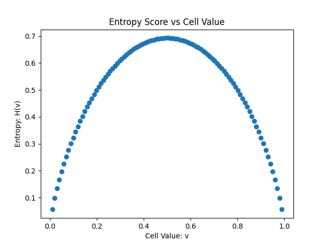
What we notice from this plot is that the highest entropy is due to cells that are unknown or a perfectly fair 50/50 probability. This means that the ternary OccupancyGrid values $[-1, 0, 100]$ can be represented as $[0.5, 0.01, 0.99]$ for unknown, free, and occupied respectively. This means that for any state $t$ we can calculate the entropy of the existing map.

For goal calculations, we calculate the expected state update $t+1$ if the robot were to be placed at each candidate location $f$ within $F = [f_1, f_2, …, f_n]$ where each $f$ is a frontier cell. Because free and occuped cells have the same entropy from being “known”, then we can further simplify the entropy calculation into a count of the location that “flips” or learns the most unknown cells. We will call this “flipping” function $U(p(x))$. If we let the set $C = [c_1, c_2,…, c_n]$ represent the set of scores $c$ associated with each candidate cell $f$, then the goal frontier $f_{goal}$ is equal to the following.

\[f_{goal} = F(c*)\]

where

\[c* = \mathop{\mathrm{arg\,min}}_{c \in C}~H(p(x))_{t+1}\]

OR where

\[c* = \mathop{\mathrm{arg\,max}}_{c \in C}~U(p(x))_{t+1}\]

Either way, so long as these functions are evaluated at the same place over the same visible area, both $U$ and $H$ will return the same $f_{goal}$.

To ensure that the calculation is realistic, the number of “flipped” cells or “learned” cells in these calculations is considered to be a circle of cells around the candidate location equivalent to the robot’s viewable radius. This radius is based on the sensor on the robot and the mapper params set in slam_toolbox, therefore it is made to be a tunable parameter. Cells that are obstructed by occupied cells will not be considered in the state update calculation as they would not be updated if the robot were present at the location.

When this algorithm is used in conjunction with DBSCAN clustering, the vector of frontiers $F$ is replaced with the vector of frontier cluster centroids and each of those is evaluated the same way.

DBSCAN Clustering

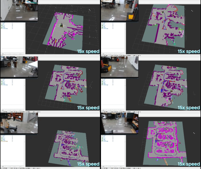
To make this work, I implemented a version of DBSCAN, formally know as “Density-Based Spatial Clustering of Applications with Noise” to cluster my frontiers. The logic flows as the following:

Input:

• eps: The maximum distance to consider two points as neighbors.
• min_samples: The minimum number of neighbors required to make a point a core point.
• points: A matrix of points (cv::Mat) where each row is a 2D point.

Steps:

1. Initialization:
   • Label all frontier cluster_ids as -1 (noise), then change the ID as they are associated with a cluster.
2. Neighbor Calculation:
   • The helper function find_neighbors calculates the indices of points within eps distance from a given point using the Euclidean distance (cv::norm) between points.
3. Logic:
   • Iterate over each point:
   • If already labeled, skip the point.
   • Find its neighbors:
     • If the number of neighbors is less than min_samples, mark the point as noise (-1).
     • Else, start a new cluster:
       • Assign the point to the current cluster ID.
       • Expand the cluster by processing its neighbors:
         • Points previously labled as noise are re-labeled as part of the current cluster.
         • Core points (neighbors with sufficient neighbors themselves) have their neighbors added to the expansion queue.
         • If two clusters with different labels have perfectly adjacent neighbors (cells are bordering) they will be merged and relabeled allowing for continuous frontiers.
4. Return:
   • A map object containing an integer referring to the cluster ID corresponding to a vector of cells associated with that ID.
5. Centroid Calculations:
   • Once the clusters have been created, the custom struct populates the centroid vectors with the cell and world coordinates for each centroid location.

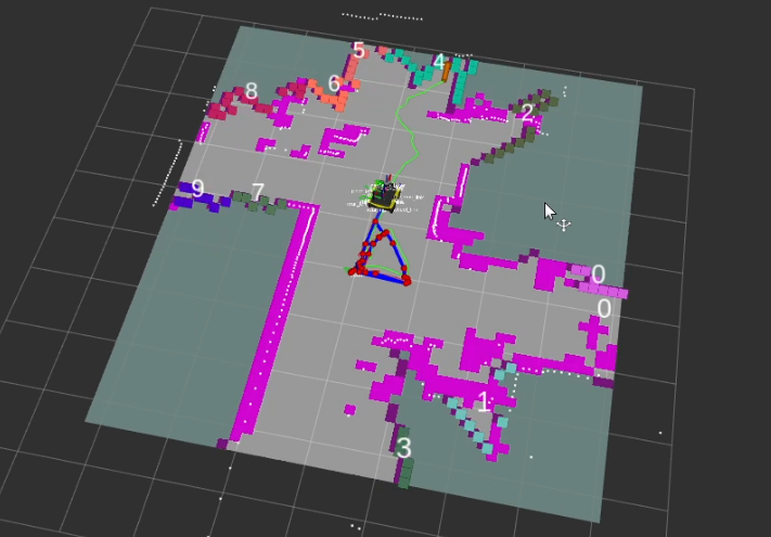
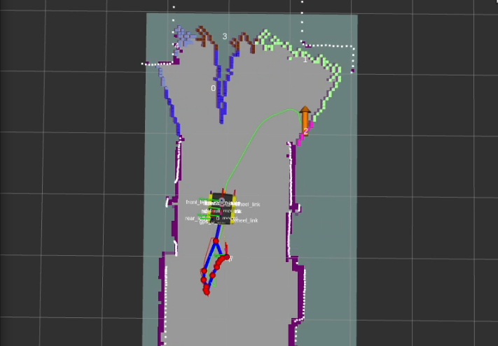
The above images show the clusters generated by the algorithm. Each cluster appears as a random color, and the number in white represents the cluster ID positioned at the centroid of the cluster.

Algorithm Comparisons and Results

By bagging the data, the learned map (known area) vs. search duration could be plotted to evaluate exploration performance. The color code is as follows:

• Orange: Single cell naive distance calc (Method 1)
• Blue: Single cell entropy calc (Method 2)
• Purple: Clustering distance based calc (Method 3)
• Green: Clustering with Entropy based calc (Method 4)
• Red: Clustering where cluster size determines goal (Method 5)

What these plots indicate is that the more “greedy” exploration algorithms performed better than those focused on longer time horizons in less cluttered or less featured spaces. More complicated areas like the lab space allowed the robot to explore areas that the greedier algorithms would miss. Selecting the closest frontiers/clusters and the largest clusters proved to be very effective ways of getting a robot to autonomously navigate without large state machines or multi-planner ensembles.

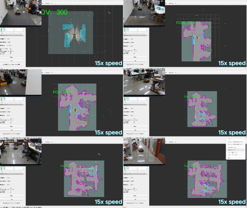
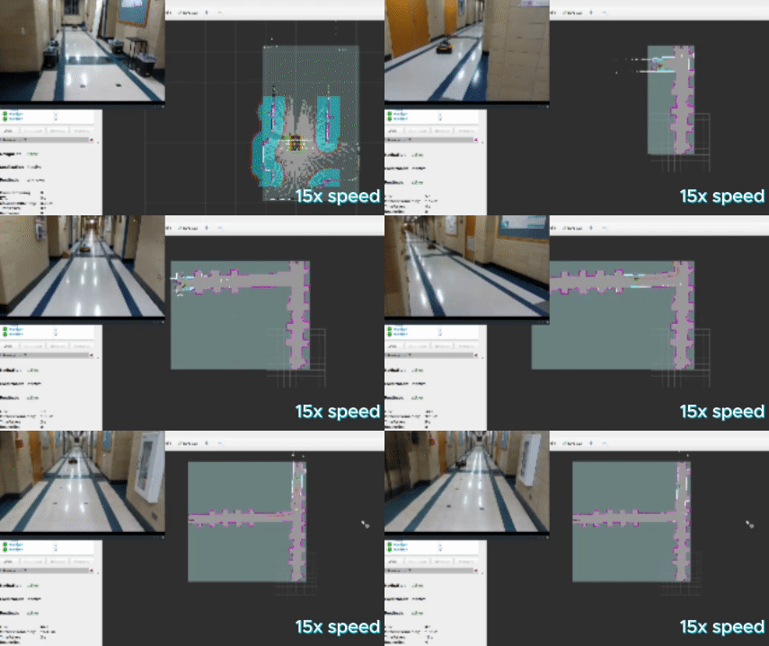
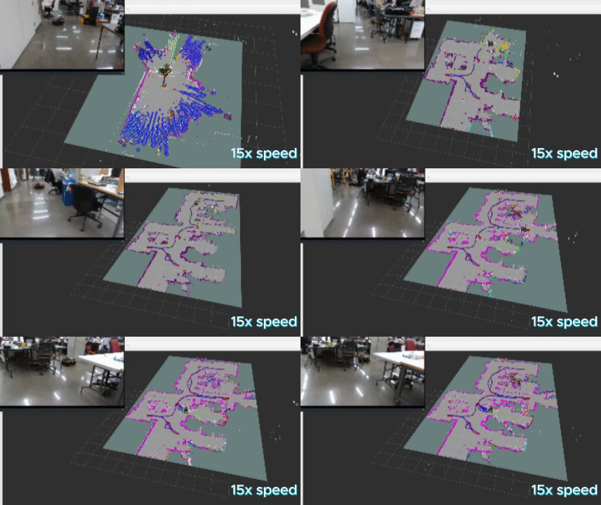
Below are a series of videos showcasing the robot’s exploration in a side-by-side manner for select algorithms. It is broken up into cluttered lab space, empty hallways, and simulated environments. Each environment presented different challenges that different pieces of my algorithms were created to address. Some of these are parameters that can be tuned in the frontier_params.yaml file based on the descriptions in the repository README.

Cluttered Lab Space

This video showcases that each algorithm was able to autonomously explore and map the environment in spite of the clutter and invalid paths created due to the clutter. The more greedy algorithms seemed to perform the fastest (as seen by the amount each video was sped up) though as the plotted data indicates, sometimes the greedy algorithms required backtracking from deep corridors.

NOTE: Due to dynamic conditions of the lab space, not all test runs provided the same area for the robot to explore.

Open 3rd Floor Hallways

In a longer, less featured space like this hallway, all algorithms performed well, though the mutual information approach showed more indecisive behavior. Due to the doubling back resulting from the indecisiveness, the algorithm was slower, but it did decided to explore both corridors which has merit. The “greedy” algorithms displayed a more depth-first approach.

Robot Setup

The robot_mapping package includes several ROS2 nodes that allow the user to run slam_toolbox with some added features. The intercept node allows the user to dynamically change the FOV of the LaserScan message for study with low sensor data cases. By simply publishing with ros2 topic pub /fov std_msgs/msg/Int64 "{data: <FOV_degrees>}" the FOV of the LaserScan can be adjusted.

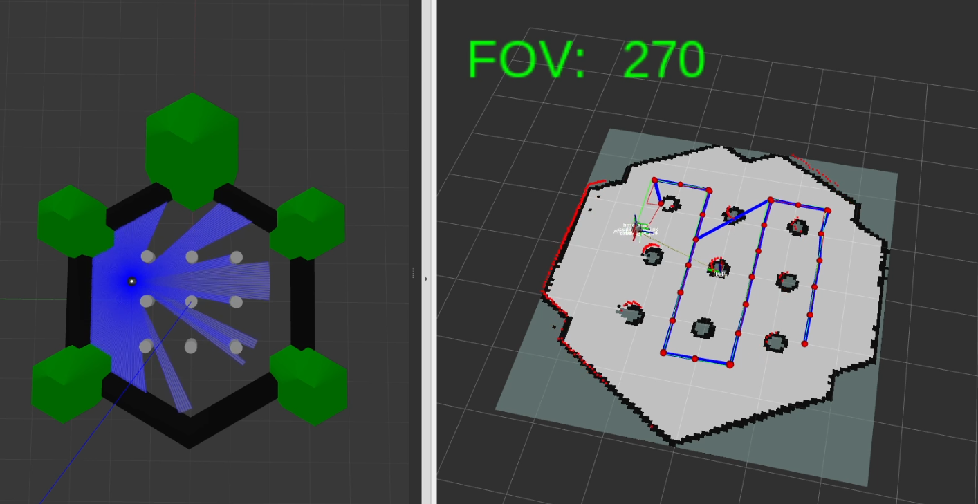
The pointcloud_to_laserscan node allows the user to easily convert 3D scans to 2D since slam_toolbox is a 2D LIDAR platform. This package also provides scripted paths for perfect repeatability in simulation.

Interfacing With Nav2

The Nav2 stack is easy to use and can be utilized by simply publishing on the /goal_pose ROS2 topic, but for further control and and a closed feedback loop, I have created a package nav_client_cpp to handle action feedback. Unlike simply publishing on the /goal_pose topic, using the services in this package allows for replanning upon failure, and diagnostic printouts. Through topics and service calls, this package can easily interface with a planner node/package. The structure is as follows:

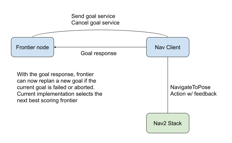
This navigation client combined with the frontier_exp_cpp and the robot_mapping packages makes deploying frontier exploration simple and approachable.

Acknowledgements!

Max Muchen Sun Project Mentor website

Matt Elwin MSR Advisor website

I would like to thank Max and Matt for their guidance and support with this project. They have taught me a lot about mathematical modeling, software architecture, and robotics testing that were invaluable in pursuing my interests in autonomous exploration.