Computer Vision Basketball Trainer

Project Goal

This project aimed at using computer vision techniques to provide feedback on a the free throw shots executed by a basketball player. By tracking the motion of the ball and motion of the player’s hands, the program outputs a PDF document offering data to help the player improve including the following:

• An overall score out of 100
• The release angle
• Graphs comparing the player’s free-throw shot to one from Steve Nash

Video Demo

Full Video Report

Final Output

Feedback

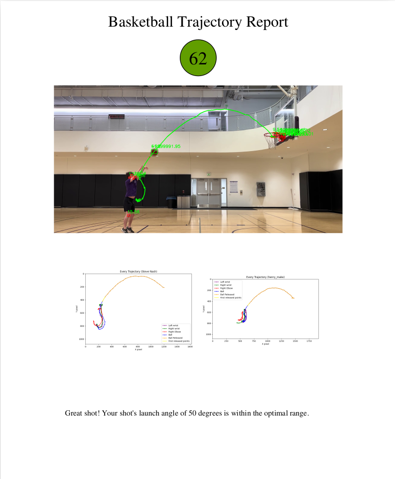
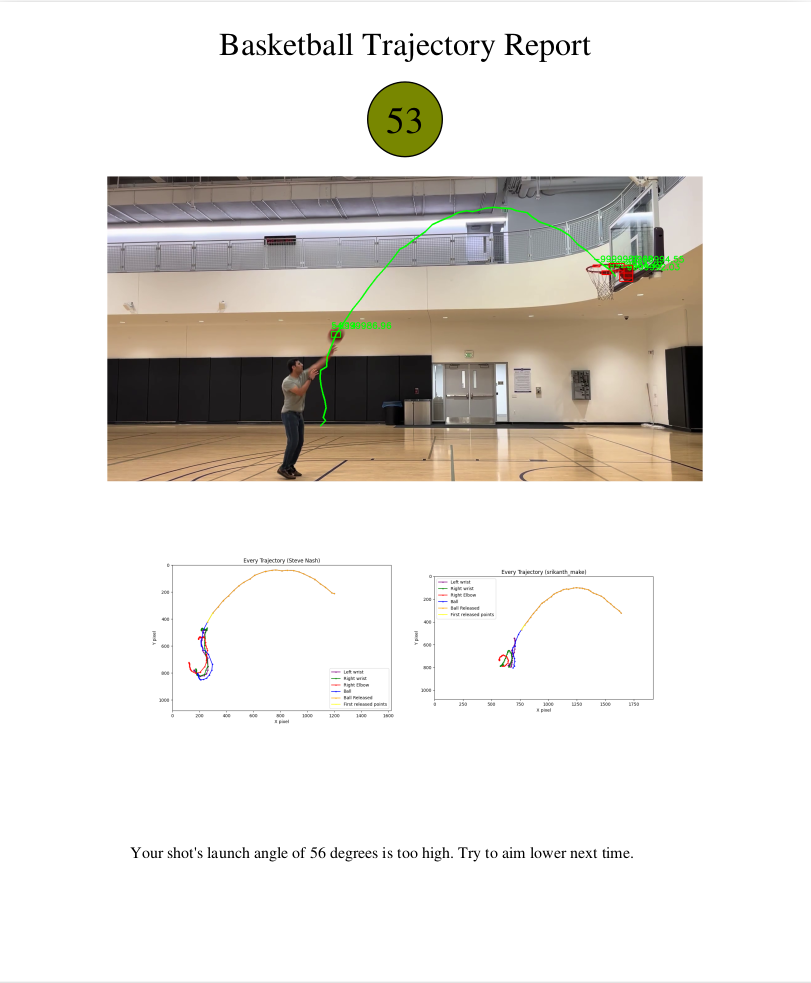
Below are examples of the final output for this project. Both are examples show that we have made the shot, but based on the analysis, Henry’s shot is a higher quality shot than mine which is reflected in the score, the feedback, and the color of the score bubble. Because my shot is too high and falls out of the optimal range, I score lower. The graphs also show that my trajectory is further from Steve Nash’s which, according to the shape analysis, will also lower my score.

Using the tracker

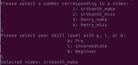
Using the program is fairly simple. A user selects the video to be assessed, and then enters their skill level from pro, intermediate or beginner. Once this is done, the program will show the mediapipe video, the ball tracking, and then generate the pdf with helpful information to improve your shot.

Tracking the Player

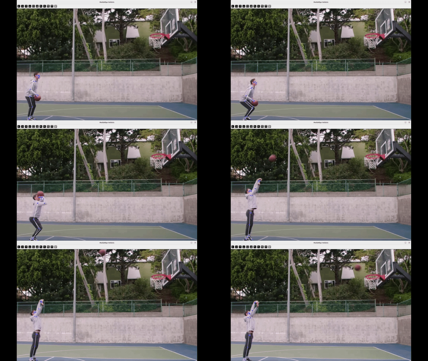
To track the motion of the player, we used Google’s Mediapipe program to get the trajectory of the key-points on the player’s body. For our analysis, we focused on the motion of the hands/wrists as the player shot the ball.

Tracking the Ball

Identifying the Ball Trajectory

Tracking the motion of the ball, unlike that of the player, proved to be a bit more complicated due to a few key challenges that often appear in computer vision applications.

• Variable Lighting Conditions
• Motion Blur
• Multiple instances of a ball in the frame
• Multiple objects of a similar color (basketball color)

To remedy these issues, the program first naively identifies all possible instances of the ball by masking each frame of the video based on the range of colors the ball could be (dark brown to bright orange). With these, each instance is rated on the following parameters and given a score:

• Squareness
• Size
• Distance from the last ball sighting

Each of these parameters is then normalized and weighted and given a total score which gives the highest likelihood of the identified “ball” being the actual basketball. The gif below shows the program tracking the ball.

As seen in the video, the naive guess identifies the actual ball, the hoop, and some of Steve’s skin as a potential ball. This is remedied by the scoring algorithm which allows for fairly accurate trajectory tracking of the ball. The red dot notes the last seen location which helps ensure that ball was properly tracked.

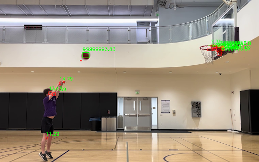
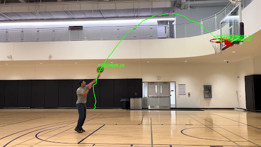
The photo of Henry on the left shows the objects identified in the frame with their scores associated. While the initial mask identifies his knees and elbows as potential ball instances, the final output is not affected. In the image to the right, a frame from my video is overlayed with the overall trajectory of the ball throughout the video. The rightmost photo of my shot trajectory shows that in spite of some noise, we can still achieve a smooth trajectory that is then added to the final output PDF.

Calculating Shot Angle

Once the trajectory of the ball is captured, calculating the release angle is relatively easy. First, the release point is calculated by plotting only the points on the ball trajectory that are more than a certain euclidean pixel distance from the hands since the hands will always be close to the ball during the shot. This threshold is usually about 40-50 pixels.

Once that set of points is extracted, then finally the first two points can be extracted from the post-release set of points to calculate the release angle using the equation Θ = tan-1(-(y2-y1)/(x2-x1)). Note that since images have the y-axis starting from top to bottom, we must flip the sign to get the proper perceived angle.

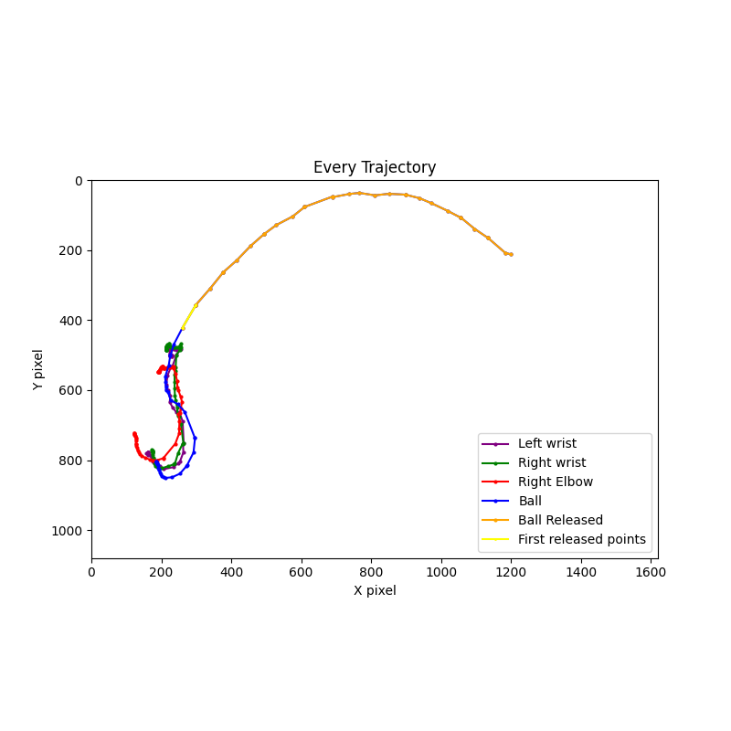
The plot above shows the various trajectories captured throughout the exploration that provide feedback to the user. This plot is the “ground truth” plot created from Steve Nash’s shot.

Comparing the Player’s and Ball’s Motion

While using Mediapipe provides the trajectory of Steve Nash’s and the player’s motion, finding a way to meaningfully compare the trajectories and represent that as a score out of 100 required some creativity. By fixing the angle of the camera to be orthogonal to the player’s shot, the number of variables is reduced, but the question of shape analysis remained unclear. To resolve this, two separate methods of trajectory shape analysis were used and combined for a total overall score.

• Fast Dynamic Time Warping (FastDTW) : A technique that measures similarity between two sequences which may vary in time or speed
• Procrustes Analysis : A statistical shape analysis method used to compare shapes involving translating, rotating, and scaling the shapes to minimize the differences between them.

While these techniques were able to provide scores, two problems remained:

1. There was no scale for the output from each scoring method
2. The scoring methods might not have a linear relationship with difference in shape (which adds difficulty to scoring)

To remedy this, the output of each method were analyzed, and then the output values were linearized and normalized so each method would produce similar scores.

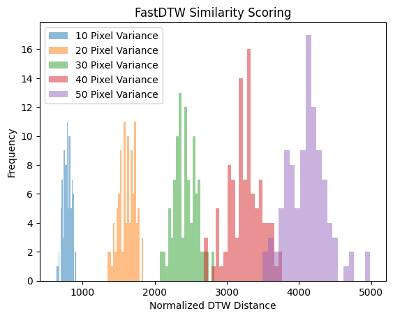
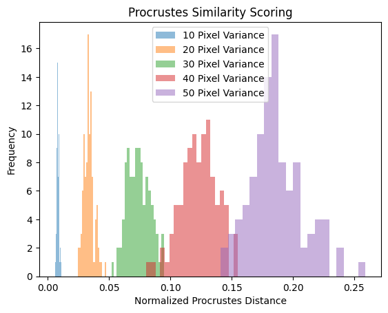
The analysis consisted of comparing an unadulterated trajectory from Steve Nash to trajectories of his with Gaussian noise added. These two trajectories were then compared and scored by both 100 times which resulted in a histogram of scores to which the mean could be assessed. To create a clear trend, the pixel variance of the noise added was increased from 10 to 50 in increments of 10 to get a full understanding of the scores.

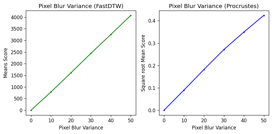
With FastDTW showing a linear relationship between mean score and blur variance and Procrustes showing a linear relationship between square root mean score and pixel blur variance, the slopes could then be extracted to assess how “off” a trajectory is on average and how much of a penalty should be deducted from 100 for it.

The final scores for FDTW and Procrustes then become:

• Final_FTDW = 100 - (FDTW/(FDTW_slope/skill))
• Final_proc = 100 - (sqrt(proc))/(proc_slope/skill)

These are then multiplied by weights, which for our case are 0.5 for each, and summed to get the final total score. If the user has chosen to identify as a beginner or intermediate, then a handicap is applied to the penalty in the form of the skill factor which is 0.1 for Beginner, 0.25 for intermediate, and 1.0 for pro (unchanged).

Taking a look at the final scoring sheet again, we can see that my score is quite low because my hand motion did not resemble the nice fish hook shape that Steve creates. We also see that my ball is creating a steeper parabola which givem me a comment to lower my release angle.

Source Code

This project was a lot of fun to work on. To view the code that we wrote for this project, please view it on GitHub! For anyone who would like to build on this project, please fork the project and try it out for yourself.

• Github Repository